Adjusting California school district relative performance for demographic differences
By Marc Joffe, Kevin Ji
Adjusting California school district relative performance for demographic differences
By Marc Joffe, Kevin Ji
Introduction
California school districts show wide variation in average test scores and graduation rates. Although school officials in high performing districts claim their performance is from their superior staff and programs, their results may instead be attributed to demographics of a district’s households. California’s statewide data platforms and accountability systems, like the California School Dashboard, also overprioritize raw performance without adjusting for structural advantages. We find that about 70% of the variance in district test performance is attributable to demographic differences across districts.
In this study, we extract demographic factors to determine which districts are, in fact, providing above-average or below-average educational services. By accounting for district demographics, we isolate the impact of the school district on student performance. Research on California’s “positive outlier” districts has demonstrated that some high-need districts consistently beat the odds, and that identifying them requires adjusting for structural advantages in districts rather than comparing raw results (Podolsky et al. 2019).
This report applies this structural adjustment to every traditional public school district in the state. We combine machine-learning and regression-based models into a single composite measure of each district’s deviation from expected performance and validate with external benchmarks. We then make profiles of several notable districts, identify why they deviate from what we expect, and give recommendations for improving the California school district data platform.
Literature Review
California has had two official iterations of a school ‘ranking’ system to track academic performance. From 1999 to 2013, California used the Academic Performance Index (API), which assigned each school a number on a scale of 200 to 1,000 depending on how well its students performed on a variety of standardized assessments (Ed-Data 2013). The API stratified results for different subgroups of students within a school, but did not incorporate variables outside of test scores. In 2014, the API was abandoned in favor of the current California School Dashboard. Since its adoption, the California School Dashboard has been criticized by researchers for metrics that obfuscate comparisons between schools and inflate the apparent performance of schools with poor subgroup results (Polikoff 2019a). Education officials and legislators have also criticized the dashboard for providing inadequate guidance on how districts can improve (CSBA 2019), and in a 2024 report, the nonpartisan Center on Reinventing Public Education gave the dashboard a “D” rating (Michel-Herf 2024). Critics have suggested the state move toward a value-added or residual-gain model that removes the effect of demographic disparities between districts in order to isolate the contribution of the district itself (Polikoff 2019b).
These controversies have prompted several third-party attempts to rank California school districts. One is GreatSchools, a nonprofit that began in California and now rates public schools across the United States, with roughly half of all K–12 households visiting the site annually (GreatSchools 2026). The nonprofit has been criticized for inadvertently exacerbating social and economic segregation, as higher-income families on average leave lower-performing schools when given GreatSchools’ information, widening performance gaps between low-income and high-income school districts (Hasan and Kumar 2018).
There have also been school performance comparisons more oriented for academics or education officials. The Stanford Educational Opportunity Project created a dashboard that allows comparisons between districts, schools, and states by standardizing results nationwide (Reardon et al. 2021). The Education Consumers Foundation has created performance charts for California districts by region, though as part of a multi-state product (Education Consumers Foundation 2024). The only tool that focuses solely on California districts is the Ed-Data comparisons tool maintained by the state’s Education Data Partnership, but its results do not isolate the value each district adds to student performance (Ed-Data, n.d.).
Think tanks and policy institutes have attempted ranking or value-added models but only to discuss California education holistically rather than compare districts. The Policy Analysis for California Education (PACE) group, whose members are faculty from the University of California and Stanford, has also analyzed the academic performance of districts across California (Kurlaender 2018), though its report focused on the state’s struggles relative to other states rather than on comparing districts within the state. The Learning Policy Institute’s “positive outliers” research took an approach closer to ours, using regression residuals to identify districts whose students of all backgrounds outperform demographic expectations (Podolsky et al. 2019).
Previous attempts to emphasize fair comparisons between California school districts are obscure. In 2011, Ira Sharenow, an independent researcher, issued a report claiming that Albany High School (AHS)—a Bay Area school normally regarded as high performing—was, in fact, a low performing facility when demographic factors were considered. Sharenow compared AHS’s API with those of other schools across California. To control for demographic differences between student bodies, Sharenow included both the English learner rate and the percentage of students on reduced/free lunch programs in a linear regression. The state discontinued publication of the API subsequent to Sharenow’s work, necessitating the use of alternative metrics.
This report adopts Sharenow’s value-added approach to currently available data and endeavors to rate all school districts rather than just one school. We directly frame our analysis around comparison between California school districts rather than other states or nationally.
Data
Our analysis draws on four public sources, all at the district level elaborated in the table below.
| Data Source | Year(s) | Variables Used |
|---|---|---|
| American Community Survey Education Tabulation (ACS-ED), National Center for Education Statistics (NCES) / U.S. Census Bureau | 2019–2023* | Adult bachelor's degree attainment, median household income, unemployment rate, poverty rate, English learner rate, free/reduced-price lunch rate |
| Ed-Data (California Department of Education Partnership) | 2024–25 | CAASPP English language arts proficiency, CAASPP mathematics proficiency, district revenues and expenditures, teacher characteristics, instructional days |
| NCES Common Core of Data (ELSi Table Generator) | 2024–25 | Noncharter enrollment, district geographic coordinates, locale classification, district type (elementary, high school, unified), staffing counts, school counts |
| California School District Areas File (California Department of Education) | 2024–25 | Differentiated Assistance status, student group counts (for ethnicity, race, English Learner, etc). Differentiated Assistance status is California’s mechanism for flagging which school districts need and receive the most support. |
Table 1. Data Sources
*: These are the most recent district-level tabulations from the ACS.
Because no single identifier spans all four sources, we joined the files from the sources in two steps. We matched Ed-Data records to NCES records on standardized district names, with a small manual correction table for districts whose names differ across systems. In the case that a district shared the same name across multiple counties, the name of the county was used to differentiate the districts. The ACS-ED and state assistance files were then merged onto the Ed-Data and NCES records using the NCES agency identifier (LEAID). This created a merged file with 991 California school districts.
We transformed and filtered the dataset to ensure all districts included were valid to rank against one another. To maintain statistical stability in accordance with the CDE’s standards, we removed all districts with under 30 enrolled noncharter students from the modelling sample. Districts classified as ‘State Board of Education Charters”, “Common Administration District”, “Statewide Benefit Charter”, or “County Office of Education (COE)” were removed from the dataset. Locale subcategories, such as “City: Large” or “City: Mid-size” were collapsed into 4 larger city, town, rural, and suburb categories. The locality categories come from the NCES Locale Classification System and are also defined in Appendix table A1 (NCES, n.d.). After filtering the dataset, 880 districts are modelled and ranked.
Since some of our statistical methods cannot handle missing values, we impute missing predictor values using scikit-learn package’s iterative imputer with a Bayesian ridge regression estimator. This iterative imputer is identical to the procedure implemented in the R language’s “mice” package (van Buuren and Groothuis-Oudshoorn 2011). Within the cross-validated machine-learning models, imputation is re-estimated inside each training fold to avoid information leaking from held-out districts. All data cleaning and analysis were performed in Python 3.13, principally with the pandas, NumPy, scikit-learn, statsmodels, PySAL (libpysal, esda, spreg), SciPy, and matplotlib packages.
| Characteristic | City (n=141) | Suburb (n=269) | Town (n=145) | Rural (n=325) | Total (n=880) |
|---|---|---|---|---|---|
| CAASPP ELA Score | 52.2 (15.5) | 53.5 (17.6) | 40.8 (11.8) | 38.1 (16.0) | 45.5 (17.3) |
| CAASPP Math Score | 41.3 (18.1) | 42.6 (20.4) | 26.6 (10.4) | 28.8 (16.0) | 34.7 (18.5) |
| Median Household Income | 112900.6 (38240.9) | 110830.0 (40556.9) | 75997.8 (23263.5) | 80444.2 (32030.0) | 94142.0 (38263.8) |
| Adults with Bachelor's % | 23.4 (8.7) | 22.6 (9.8) | 14.4 (7.5) | 15.6 (8.4) | 18.8 (9.6) |
| Unemployment % | 5.9 (1.8) | 6.0 (1.8) | 8.1 (3.9) | 8.0 (5.4) | 7.1 (4.0) |
| Poverty % | 7.5 (4.1) | 7.4 (4.4) | 11.6 (6.4) | 9.9 (8.8) | 9.0 (6.8) |
| Free/Reduced Meal % | 54.7 (24.3) | 53.2 (27.6) | 67.9 (18.7) | 59.3 (22.1) | 58.1 (24.3) |
| English Learners % | 19.8 (12.1) | 15.0 (10.5) | 18.7 (14.6) | 15.4 (15.7) | 16.6 (13.6) |
| Disabled Student % | 13.5 (2.4) | 13.6 (2.8) | 13.8 (3.2) | 13.2 (4.7) | 13.5 (3.6) |
| Ethnic Diversity Index | 40.0 (15.7) | 38.7 (15.6) | 29.9 (16.4) | 31.3 (13.4) | 34.7 (15.5) |
| Log Enrollment (Non-Charter) | 9.1 (1.1) | 8.5 (1.2) | 7.4 (0.9) | 5.6 (1.1) | 7.4 (1.8) |
| Teaching Days | 180.2 (1.1) | 180.2 (0.9) | 180.2 (0.8) | 179.3 (11.7) | 179.9 (6.7) |
| District Type: Elementary % | 45.4% | 43.1% | 39.3% | 69.5% | 52.6% |
| District Type: High School % | 15.6% | 7.8% | 14.5% | 3.7% | 8.6% |
| District Type: Unified % | 39.0% | 49.1% | 46.2% | 26.8% | 38.8% |
Table 2. School district characteristics.
Note: Numbers are means, values in parentheses represent standard deviations (SD).
Methods
This section describes the models in plain terms. More technical detail is provided in the technical appendix. Much of the work is based on the technical appendix of the Stanford Data Education Archive.
The goal of our models is to predict each district’s test results from its demographic characteristics, and treat the gap between actual and predicted results (residuals) as the isolated impact of the district. The outcome variables are the percentage of noncharter students meeting or exceeding standards on the CAASPP English language arts (ELA) and mathematics assessments. Outliers are a severe threat to creating a stable ranking system. To stabilize the rankings, our design fits several models, averages them, and applies both shrinkage and smoothing techniques to the residuals to minimize statistical distortion from outlier districts.
Three Models
Three models were fit before being combined, an ordinary least squares (OLS) model to capture linear relationships, an elastic net model to remove highly correlated predictors, and random forests to capture non-linear relationships. To prevent overfitting, each model’s out-of-sample accuracy was estimated with five-fold cross-validation. For reproducibility, a consistent seed was set for all models. By using cross validation, we ensure that other researchers can apply this ranking system to new school districts or new test score results.
We fit each model with the same set of predictors and all predictors were chosen based on precedent in education policy literature. To account for the demographics of the area surrounding the district, we included district demographics like bachelor percentage and median income. To control for the enrolled student population, we included variables such as free/reduced lunch rate and English learner rate. Finally, we also accounted for structural factors such as how rural the district is or the category of the district (unified/high school/elementary).
The random forest and ordinary least square models explain roughly 70% of the district-to-district variation in ELA proficiency and roughly three-quarters of the variation in math proficiency out of sample. The elastic net model only explains roughly 40% of the variation in test scores between districts (Appendix Table B3).
Combining models
The three model families and two subjects yield six residuals for each district (random forest math, OLS math, elastic net math, etc) each standardized as a z-score. We combine the residuals through a weighted average to create a composite score for the district. Rather than giving every model equal weight, we use principal component analysis to determine how much weight each model should receive based on the information it contributes. Several adjustments were made to the composite z-score to minimize the influence of outliers (Appendix section C).
Tiny districts are structurally much more likely to have outlier test scores that are not indicative of the district’s actual teaching ability. A reasonable model of district performance should be more skeptical of a smaller district since it is easier for scandals or extraordinary circumstances in one school to affect the entire district. To incorporate this assumption, we shrink small district residuals based on the size of the noncharter population and whether the district is located in a rural, suburb, town, or city. The smaller the district, the more its estimate reverts to the mean of its locality. This process is formally known as empirical Bayes shrinkage and is elaborated in Appendix section D.
Neighboring districts share labor markets, housing patterns, and county offices of education, so their results may be correlated beyond what our predictors predict. We ran a diagnostic on the baseline regression residuals to identify spatial correlation. Each district’s eight nearest neighbors (by euclidean distance between districts) were identified and weighted by inverse distance, so that closer neighbors count more. A Moran’s I test on the residuals indicates that spatial correlation in both English and math results is statistically detectable but small in magnitude (Appendix Table C1), which shows that the predictors in the baseline model already absorb most geographic clustering.
After empirical Bayes shrinkage, we adjusted for the natural correlation in test scores between neighboring districts. For each of the six residual scores, a spatial autoregressive (SAR) model estimated how strongly a district’s performance correlates with its neighbors’ performance. Each district’s score becomes a weighted average of its own residual and the average of its eight neighbors’ residuals. The estimated weights assign roughly 60% of a district’s performance to the district itself and roughly 40% to its neighboring districts (Appendix Table C2).
Assigning tiers
A reliable ranking system requires that the rankings for each district remain stable between different models. To quantify ranking stability, we repeatedly simulated plausible versions of the rankings based on each district’s estimated statistical uncertainty (Appendix section E). We performed 1,000,000 simulations, and the 2.5th and 97.5th percentiles of each district’s simulated ranks form a 95% stability interval around its published rank.
All school districts were ranked and sorted into 5 tiers. These five tiers are based on the composite score: Significant Overperformer, Moderate Overperformer, Expected Performer, Moderate Underperformer, and Significant Underperformer (tier definitions in appendix table F1). For robustness, we compared the similarity of rankings of our model averaged design and an unmodified regression model using a Spearman rank correlation test and found they had a high 0.87 correlation.
Results
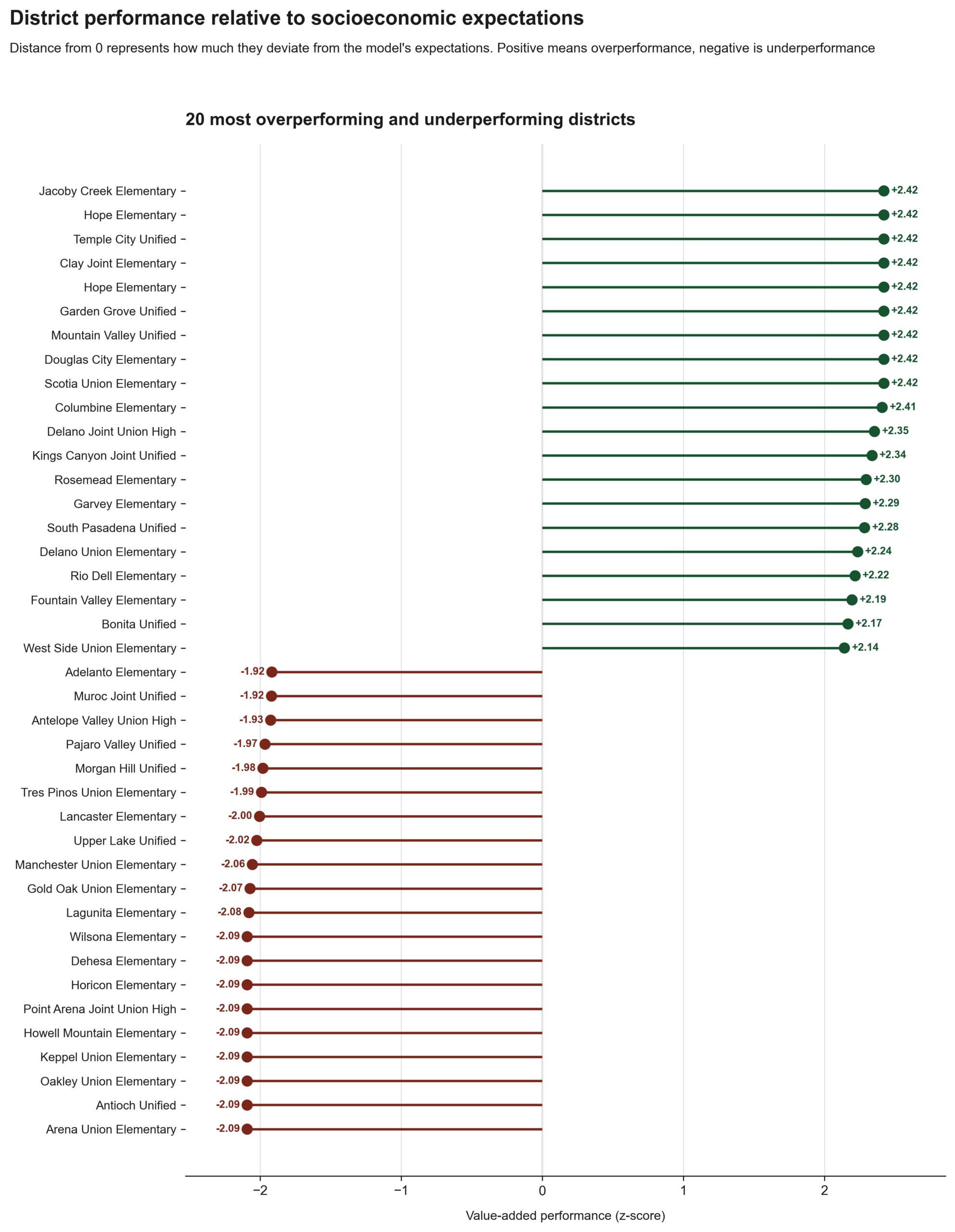
Across the 880 ranked districts, 69 are Significant Overperformers, 198 Moderate Overperformers, 328 Expected Performers, 230 Moderate Underperformers, and 55 Significant Underperformers. The further a district sits from the middle of the distribution, the more stable its ranking proved in the simulations: Garden Grove Unified and Campbell Union, the best and worst-ranked districts respectively, had 95% stability intervals of roughly five spots. Across 1 million simulations, their 2.5th and 97.5th percentiles of those simulations only deviated by about 12 spots. Districts near the median, by contrast, swung enormously between simulations. Grass Valley Elementary’s interval spans 189 positions in either direction and Buttonwillow Union spans about 299 positions. The population of the school district also affects the ranking stability and as expected, larger districts had a much higher ranking stability.
High school districts were often Expected Performers while small elementary districts dominate the extremes of the distribution. The smallest districts in our ranked sample were most prevalent in the extreme tiers, partly because a scandal or an excellent teacher or principal can disproportionately affect a smaller student body. Even with the shrinkage techniques deployed against this, it remains structurally easier for small districts to succeed or fail dramatically. Thus, comparisons between small and large districts should still be made with caution.
In the next two sections we profile several districts among the extreme overperformers and underperformers in our data set. This analysis can help us better understand why school districts are relatively successful or unsuccessful in educating their students once demographic factors are removed.
Notable Overperformers
Compton Unified
Compton Unified, previously notorious for its academic struggles, has made dramatic improvements in test scores and graduation rates since the pandemic (Bell 2025). Over its lifespan, the district has endured a state takeover, financial bankruptcy, and chronically low achievement (Mathews 2000). Even though over 95% of its student body is classified as high-need, it has raised both average math and English scores by roughly three grade levels, now matching the statewide average (Seshadri 2025). Despite its size, it ranks within our top ten overperforming districts. Local reporting attributes the turnaround to frequent formative assessments and a requirement that each principal submit accountability and action plans for his or her own school (Seshadri 2025). The superintendent, Darin Brawley, believes the “establishment of smart goals, implementation of interventions in classrooms, and a focus on academic language for taking tests” were key to consistent yearly improvement (Riddell 2025).
Garden Grove Unified
Garden Grove Unified is a large district of roughly 37,000 students that thrives despite serving a diverse, high-need population. Within our ranking, it is the 7th most overperforming school district. Its elementary and secondary schools earn a disproportionate share of California Distinguished School awards: in 2026, Garden Grove had the third-highest number of awards among all districts (CDE 2026), and in 2025 it had the second-highest—behind only Los Angeles Unified, a district more than ten times its size (CDE 2025). Garden Grove also shared, with eight other large California districts in the CORE Data Collaborative, the Carnegie Foundation’s 2026 Award for Impact for its work improving ninth-grade on-track rates, a critical lever for graduation (Carnegie Foundation 2026).
Kings Canyon Joint Unified
Kings Canyon posts roughly 42% math and 56% reading proficiency, above the state marks, even though its student body is 88% Hispanic and 63% economically disadvantaged. State awards corroborate their success. Reedley High has twice been named a California Distinguished School, one of only a handful of traditional high schools so honored across Madera, Tulare, and Fresno counties, and Reedley Middle College High has earned the distinction three times since 2021 (CDE, 2026). Unlike other overperformers, Kings Canyon has equally overperformed both in its math and English scores by 17 and 16 points respectively. Overperformance in our dataset is typically concentrated in English scores and the state overall has focused on literacy to the detriment of math proficiency (Huffaker, 2026).
Chaffey Joint Union High
Chaffey Joint Union is one of the largest high school districts in California, serving over 22,000 high need students. 87% of its students are non-white (a majority Hispanic) and 66% are eligible for free or reduced-price meals. Our model predicted that 51.3% of Chaffey’s students would meet standards on the CAASPP English test. In reality the district beat that prediction by 17 points, and its raw proficiency rate of 68.1% places it in the top fifth of California districts for English proficiency. The model’s modest prediction was driven largely by the district’s 8% English learner share and low 18.6% adult bachelor’s attainment rate. What makes the result more impressive is that Chaffey overperforms without overspending: its current expense of $18,946 per student in 2024–25 is well below the average of roughly $22,300 across the districts in our sample.
Notable Underperformers
Saint Helena Unified
Saint Helena Unified spent $39,536 on each student in the 24-25 FY while its neighboring district, Napa Valley Unified only spent $17,390 per student in the same period. Its class sizes are also much smaller than the average California school district, with only 13.3 pupils per teacher. Located in the winemaking center of Napa Valley, this district in theory should have an abundance of local funding that pushes it beyond the state average. In spite of these advantages, local reporting shows that Saint Helena and other neighboring districts generally lag behind state standards. Compared to what our model predicts, the district falls 1.5 points short in English and 7 points short in math. Normally, underperformance is explained through scandals, disasters, or neighboring crime rates. However, there are no notable stories about the district within the last 5 years and Saint Helena as a city has a very low crime rate. A probable explanation is that since the private school enrollment rate in the area is 2.4x higher than the state average, affluent students are not enrolling in Saint Helena but cause a greater demographic penalty in the model (Private School Review, 2025).
Antioch Unified
Antioch Unified’s financial pressures and tumultuous leadership have likely led to the district’s underperformance. In 2026, the district rejected budget cuts during its financial crisis which led the county to downgrade its budget certification rating twice (Kennedy 2026). The district’s previous superintendent, Stephanie Anello, was embroiled in a year-long scandal and terminated for “failing to hold a mid-level boss accountable for allegedly bullying subordinates” (Nguyen 2024). The local community has expressed concern about Anello’s replacement, writing to the board that the new “superintendent may be deliberately hiding expenses from the board and the public” (CCNews 2026). Based on our model, the district has a 14 point underperformance in English and a 15 point underperformance in math proficiency which is likely caused by the recent scandals in the district.
Vallejo City Unified
Vallejo has been under state control for decades due to financial mismanagement, only exiting receivership in 2025 (Local News Matters 2025). Even though its high need demographics would already imply lower performance, the two decades of state receivership has left it even worse than its demographics would suggest. 74.0% of students have failed the standardized English exam and 80.9% have failed the math exam. Our model suggests that this is an underperformance of 15 points for English and 11 points for math respectively. This result is in line with studies done on district takeovers: state takeovers of districts are not found to increase academic performance and are detrimental to test scores in early years of the takeover (Schueler, 2021). Vallejo retained some local control, but the takeover resulted in frustration over transparency behind school closure decisions (Haber, 2026).
Natomas Unified
Natomas Unified’s underperformance is driven by achievement gaps between different groups. At Natomas, only 23% of Black students are meeting sufficient English standards and 13% are meeting math standards. For other demographics at Natomas, exam results are 20-40% higher. Black students are only 15% behind other demographics in statewide averages (EdSource, 2025). These results have led local parents to form the Natomas Black Parents United group in 2020, which advocates for interventions such as lowering student-teacher ratios and moving back to phonics-based instruction (Kwapo, 2025). Momentum is growing behind the parent group, which now numbers over 250 parents. In the coming years, we may see a similar comeback that Compton Unified experienced.
Trends across districts
Individual school districts are worth exploring from an accountability perspective, but the overall performance results reveal systematic trends. The table of large overperformers and underperformers shows key differences. On average, underperformers are more rural, have smaller student bodies, have less bachelor’s degree attainment for all adults in the district, and have a higher share of English learners. The ethnic diversity was almost identical between overperforming and underperforming districts.
| Characteristic | Overperformers (n=267) | Underperformers (n=276) |
|---|---|---|
| Rural Districts (%) | 32.2 | 43.8 |
| Average Enrollment | 8613.0 | 5823.0 |
| Ethnic Diversity Index | 35.1 | 34.4 |
| English Learners (%) | 14.5 | 19.1 |
| Free/Reduced Meals (%) | 52.3 | 62.9 |
| Adults with Bachelor's Degree (%) | 21.3 | 16.9 |
Table 3. Characteristics of over- and underperformers. Numbers are means.
The demographics comparison changes when the moderate overperformers and underperformers are excluded. Extreme underperformers have larger student bodies than the overperformers and the difference in demographics is more extreme compared to moderate overperformers and underperformers.
| Characteristic | Significant Overperformers (n=58) | Significant Underperformers (n=59) |
|---|---|---|
| Rural Districts (%) | 41.4 | 61.0 |
| Average Enrollment | 4338.0 | 4482.0 |
| Ethnic Diversity Index | 35.4 | 35.5 |
| English Learners (%) | 15.4 | 16.8 |
| Free/Reduced Meals (%) | 54.5 | 57.8 |
| Adults with Bachelor's Degree (%) | 19.5 | 17.6 |
Table 3. Characteristics of extreme over- and underperformers.
There was no obvious spatial correlation between counties and tiered district performances. However, when the school districts were grouped by economic regions in California, there were clear gaps in performance.

Orange County and Los Angeles County which are denser, urban counties have higher concentrations of overperformers. The more rural regions such as Kern, North State, and Central Coast have a much larger share of underperforming districts. A notable exception is the non-rural Inland Empire, which likely struggles due to high poverty areas like San Bernardino and Coachella Valley.
Model Validation
To externally validate the results of our model, we turned to Differentiated Assistance status. An unsuccessful model would have all the underperforming schools receive Differentiated Assistance from California state while the overperforming schools would have little to no Differentiated Assistance. Our data shows that extreme overperformers had lower chances of receiving Differentiated Assistance but it remained prevalent through all tiers.
| Performance Tier | Differentiated | % Differentiated | General | Total |
|---|---|---|---|---|
| Moderate Underperformer | 155.0 | 71.4% | 62.0 | 217.0 |
| Expected Performer | 234.0 | 69.4% | 103.0 | 337.0 |
| Moderate Overperformer | 112.0 | 53.6% | 97.0 | 209.0 |
| Significant Underperformer | 36.0 | 61.0% | 23.0 | 59.0 |
| Significant Overperformer | 22.0 | 37.9% | 36.0 | 58.0 |
| Total | 559.0 | 63.5% | 321.0 | 880.0 |
Table 4. District assistance status by performance tier.
Rows ordered by percentage receiving Differentiated Assistance.Another way of externally validating the results would be to see if our overperforming schools have a statistically larger share of distinguished school awards. Using awardee data for California’s Distinguished Schools for 2024 and 20251, we perform a Kendall Tau-b test to determine correlation between the ranking of a school district’s overperformance and the number of awards they received in this timespan (Appendix Table G1). Since many districts or schools had 0 awards, the Kendall Tau-B was used to adjust for the number of ties in the ranking. The p-value for our rank correlation was extremely close to 0 and the strength of the correlation was 0.21. Given that most districts receive 0 awards and that the award requires schools to apply to receive it, a correlation of this size is impressive given how noisy the validation mechanism is. The California’s Distinguished Schools Award has some overlap with our model performance criteria but the correlation strength suggests that the model is successfully identifying strong school districts.
Footnote
- Data for two years is used as elementary schools and high schools are granted the award in alternating years.
Conclusion
After stripping away structural advantages, district effectiveness varies widely across California. Districts such as Compton, Garden Grove, Kings Canyon, and Chaffey demonstrate that high-need student populations are not incompatible with strong academic performance, while districts such as Saint Helena demonstrate that districts with abundant funding and small class sizes can still fail to capitalize on their advantages.
While a district’s deviation from our model’s expectations is important, raw test score performance is still necessary for understanding a school district’s performance. An overperforming district may still broadly fail to meet state benchmarks, and an underperforming district in a high-socioeconomic area may still post strong raw results. Our tiers and rankings of the school districts should be read alongside raw test score proficiency, not instead of them.
The state should consider prioritizing demographically adjusted comparisons within the California School Dashboard and within the accountability mechanism. The dashboard does include these comparisons but they are buried beneath other measures and are not used to determine California’s accountability mechanism. Researchers have urged the state toward growth and residual-gain models for years (Polikoff 2019b). This report demonstrates that a credible statewide version can be built entirely from data the state already collects.
Rural underperformance also indicates that these districts require additional support or intervention. The bulk of the most extreme underperformers in California are in rural areas, and this trend persists after controlling for demographic factors, pointing to structural challenges that uniform state programs cannot address.
A more systematic effort to dissect what the top tier of schools does differently would convert these rankings into a roadmap for improving districts with similar demographics.The analysis has limits that future work should address. It is a cross-sectional study rather than a time series, and the district profiles are suggestive of causes but are not necessarily causal. Our profiles of notable school districts are limited based on publicly available school districts. California should invest in ground level studies or investigations of these school districts to fully understand these successes and failures. Future work should extend the framework to multiple years of data to improve robustness and incorporate student-level growth measures where available.
References
Bell, Gerald. 2025. “Once Troubled, Now Triumphant: Compton Unified Sets New Standard in Student Success.” LA Focus. July 4, 2025. https://www.lafocusnews.com/news/once-troubled-now-triumphant-compton-unified-sets-new-standard-in-student-success-818db908
Bruno, Paul. 2026. “District Dollars 3: Recent Patterns in California School District Finances, Trends in Teacher Compensation, and Within-District, Between-School Spending | Getting Down to Facts.” Gettingdowntofacts.Com. May 7, 2026. https://gettingdowntofacts.com/reports/district-dollars-3-recent-patterns-california-school-district-finances-trends-teacher
Buuren, Stef van, and Karin Groothuis-Oudshoorn. 2011. “Mice: Multivariate Imputation by Chained Equations in R.” Journal of Statistical Software 45 (3). https://doi.org/10.18637/jss.v045.i03
Carnegie Foundation. 2026. “CORE Districts’ BTSC: 2026 Carnegie Award for Impact Recipient – Carnegie Foundation for the Advancement of Teaching.” Carnegie Foundation for the Advancement of Teaching. May 11, 2026. https://www.carnegiefoundation.org/core-districts-btsc-2026-carnegie-award-for-impact-recipient/
CC News. 2026. “Letter: Concerns Expressed Over Antioch Unified Superintendent, Direction of District.” Contra Costa News. May 27, 2026. https://contracosta.news/2026/05/27/letter-concerns-expressed-over-antioch-unified-superintendent-direction-of-district/
CDE. 2025. “California Distinguished Schools Awardees.” Ca.Gov. 2025. https://www.cde.ca.gov/ta/sr/cs/distschools.asp
CDE. 2026. “State Superintendent Tony Thurmond Announces 2026 California Distinguished Schools.” Ca.Gov. 2026. https://www.cde.ca.gov/nr/ne/yr26/yr26rel12.asp
CSBA. 2019. “State Must Improve the California School Dashboard, Not Move the Goalposts.” California School Boards Association. January 4, 2019. https://publications.csba.org/california-school-news/february-2018/state-must-improve-the-california-school-dashboard-not-move-the-goalposts/
EdData. 2013. “Understanding the Academic Performance Index (API).” EdData. 2013. https://www.ed-data.org/article/Understanding-the-Academic-Performance-Index-(API)
Ellis, Anya. 2025. “Clovis Unified Boasts Increased Enrollment, High Test Scores, and New $600 Million Campus.” GV Wire. October 2, 2025. https://gvwire.com/2025/10/02/clovis-unified-boasts-increased-enrollment-high-test-scores-and-new-600-million-campus/ .
Ferrare, Joseph J, R Joseph Waddington, Ron Zimmer, and Mark Berends. 2025. “The Impacts of Virtual Charter High Schools on Secondary and Postsecondary Outcomes: Opening Up the Black Box.” Educational Researcher 54 (8). https://doi.org/10.3102/0013189×251337417
GreatSchools. 2026. “About GreatSchools.Org.” Parenting. 2026. https://www.greatschools.org/gk/about/
Guinan, Brett, and Julien Lafortune. 2025. “Exploring Record-High Student Homelessness.” Public Policy Institute of California. July 9, 2025. https://www.ppic.org/blog/exploring-record-high-student-homelessness/
Hasan, Sharique, and Anuj Kumar. 2018. “Digitization and Divergence: Online School Ratings and Segregation in America.” SSRN Electronic Journal. https://doi.org/10.2139/ssrn.3265316
k16collaborative. 2026. “Community Economic Resilience Fund (CERF) Economic Regions Map – Regional K-16 Education.” K16collaborative.Org. 2026. https://k16collaborative.org/regional-map/
Kennedy, Samantha. 2026. “Antioch Unified Fails to Pass $18.7 Million in Cuts.” The Contra Costa Pulse | Community News and Youth Voices for Contra Costa County. May 8, 2026. https://ccpulse.org/2026/05/08/antioch-unified-fails-to-pass-18-7-million-in-cuts/
Kurlaender, Michal. 2018. “PACE – Outcomes and Demographics of California’s Schools.” Policy Analysis for California Education. September 2018. https://edpolicyinca.org/publications/outcomes-and-demographics-californias-schools
Loeb, Susanna. 2026. “Toward a Stronger Next Generation of California Education.” https://gettingdowntofacts.com/sites/default/files/Toward%20a%20Stronger%20Next%20Generation%20of%20California%20Education.pdf
Mathews, Joe. 2000. “State to End Takeover of Compton Schools.” Los Angeles Times. September 18, 2000. https://www.latimes.com/archives/la-xpm-2000-sep-18-mn-23004-story.html
Medina, Madilynne. 2025. “Massive $600M School Opens in Central Valley amid Growing Population.” Sfgate. August 19, 2025. https://www.sfgate.com/centralcalifornia/article/new-school-opens-central-valley-20824475.php
Michel-Herf, Nadja. 2024. “State Secrets: How Transparent Are State School Report Cards About the Effects of COVID? – Center on Reinventing Public Education.” Center on Reinventing Public Education. September 5, 2024. https://crpe.org/transparent-state-report-card-grades-2024/
Murphy, Patrick, and Jennifer Paluch. 2018. “Financing California’s Public Schools – Public Policy Institute of California.” Public Policy Institute of California. 2018. https://www.ppic.org/publication/financing-californias-public-schools/
National Center for Education Statistics. n.d. “Locale Definitions.” Education Across America: Cities, Suburbs, Towns, and Rural Areas. U.S. Department of Education. Accessed July 30, 2026. https://nces.ed.gov/surveys/annualreports/topical-studies/locale/definitions.
Nguyen, Candice, and Jeremy Carroll. 2024. “Antioch Unified School District Superintendent Terminated amid Bullying Scandal.” NBC Bay Area. August 21, 2024. https://www.nbcbayarea.com/news/local/east-bay/antioch-unified-school-district-superintendent-terminated/3631948/.
“PACE – TK–12 Education Governance in California.” 2025. Policy Analysis for California Education. December 2025. https://edpolicyinca.org/publications/tk-12-education-governance-california.
Palmer, Riley. 2024. “Napa Student Performance Results Trail California Marks, with Surprising Takeaways.” The Napa Valley Register. November 23, 2024. https://napavalleyregister.com/news/local/education/napa-valley-unified-school-district-test-scores-caaspp-mayacamas/article_018f2d06-a875-11ef-b8d0-3be539d1d1e9.html#tncms-source=signup&tncms-source=login
Podolsky, Anne, Linda Darling-Hammond, Christopher Doss, and Sean Reardon. 2019. “California’s Positive Outliers: Districts Beating the Odds.” Learning Policy Institute. May 2019. https://learningpolicyinstitute.org/product/positive-outliers-districts-beating-odds-report
Polikoff, Morgan. 2019. “PACE – Gauging the Revised California School Dashboard.” Policy Analysis for California Education. February 2019. https://edpolicyinca.org/publications/gauging-revised-california-school-dashboard
“Radware Captcha Page.” 2026a. Ca.Gov. 2026a. https://www.cde.ca.gov/ta/ac/cm/ela24.asp
“Research Briefs – Student Success | Getting Down to Facts II.” 2026b. Gettingdowntofacts.Com. 2026b. https://gettingdowntofacts.com/research-briefs
Riddell, Roger. 2025. “How Longevity Led to Achievement Gains in Compton USD.” K-12 Dive. October 23, 2025. https://www.k12dive.com/news/lessons-in-leadership-longevity-achievement-gains-compton/803169/
Schueler, Beth E., and Joshua F. Bleiberg. 2021. “Evaluating Education Governance: Does State Takeover of School Districts Affect Student Achievement?.” Journal of Policy Analysis and Management 41 (1). https://doi.org/10.1002/pam.22338
Seshadri, Mallika. 2025. “How Compton Unified Boosted Its Standardized Test Scores.” EdSource. February 11, 2025. https://edsource.org/2025/how-compton-unified-boosted-its-standardized-test-scores/726655
Tu, Yundong, and Tae-Hwy Lee. 2019. “Forecasting Using Supervised Factor Models.” Journal of Management Science and Engineering 4 (1): 12–27. https://doi.org/10.1016/j.jmse.2019.03.001
Ugo, Iwunze , and Eric Assan. 2025. “California’s K–12 Test Scores.” Public Policy Institute of California. June 17, 2025. https://www.ppic.org/publication/californias-k-12-test-scores/
Xie, Yuxuan. 2025. “A Look at Student Poverty through Free or Reduced-Price Meal Eligibility in California Schools.” EdSource. November 3, 2025. https://edsource.org/2025/snap-funding-school-meals/744305
Technical Appendix
This appendix documents the analytical methodology and modeling pipeline implemented in the accompanying code. This section formalizes the model specifications, shrinkage estimators, and validation procedures. Section letters correspond to references in the main text.
A. Data Sources and Merge Procedure
The analysis leverages five integrated data sets spanning fiscal year 2024-25 and the 2019-2023 ACS periods: (1) Ed-Data district-level performance, staffing, and finance extracts; (2) the NCES ELSi district table; (3) NCES ACS-ED district tabulations; (4) the CDE California School District Areas file; and (5) the CDE California Distinguished Schools awardee roster for external validation. The original merged dataset, before filtering, has 191 columns and 990 rows.
Ed-Data and NCES records were matched utilizing standardized string algorithms applied to district names. Economic and demographic covariates from the ACS-ED were joined via the unique NCES local education agency identifier (LEAID). To ensure comparability, State Board of Education Charters, Common Administration Districts, Statewide Benefit Charters, and County Offices of Education were excluded from the sample.
Table A1. NCES Locale Classifications and Criteria
| Locale Code | Locale | Subtype | Definition |
|---|---|---|---|
| 11 | City | Large | Territory inside an urbanized area and inside a principal city with population of 250,000 or more |
| 12 | City | Midsize | Territory inside an urbanized area and inside a principal city with population less than 250,000 and greater than or equal to 100,000 |
| 13 | City | Small | Territory inside an urbanized area and inside a principal city with population less than 100,000 |
| 21 | Suburban | Large | Territory outside a principal city and inside an urbanized area with population of 250,000 or more |
| 22 | Suburban | Midsize | Territory outside a principal city and inside an urbanized area with population less than 250,000 and greater than or equal to 100,000 |
| 23 | Suburban | Small | Territory outside a principal city and inside an urbanized area with population less than 100,000 |
| 31 | Town | Fringe | Territory inside an urban cluster that is less than or equal to 10 miles from an urbanized area |
| 32 | Town | Distant | Territory inside an urban cluster that is more than 10 miles and less than or equal to 35 miles from an urbanized area |
| 33 | Town | Remote | Territory inside an urban cluster that is more than 35 miles from an urbanized area |
| 41 | Rural | Fringe | Census-defined rural territory that is less than or equal to 5 miles from an urbanized area, as well as rural territory that is less than or equal to 2.5 miles from an urban cluster |
| 42 | Rural | Distant | Census-defined rural territory that is more than 5 miles but less than or equal to 25 miles from an urbanized area, as well as rural territory that is more than 2.5 miles but less than or equal to 10 miles from an urban cluster |
| 43 | Rural | Remote | Census-defined rural territory that is more than 25 miles from an urbanized area and also more than 10 miles from an urban cluster |
B. Model Specifications
Let Ydb denote the observed proportion of students meeting or exceeding standards in district d for subject b ∈ {ELA, Math}. We estimate the expected achievement based on a vector of district-level demographic and structural covariates, denoted Xd. We implement three distinct model families to predict Ydb: Ordinary Least Squares (OLS), Elastic Net Regularization, and Random Forest. The models are estimated on the restricted sample of districts that possess valid achievement data, geographic coordinates, and standardized identifiers.
B.1 Covariate Imputation
Prior to estimation, missing continuous covariates in Xd are imputed using an iterative, multiple-imputation framework utilizing scikit-learn’s Bayesian Ridge Regression estimator. Missing categorical covariates (e.g., locale code) are assigned the sample mode. In regard to imputation for cross-validation, the imputation process is re-estimated strictly within each training fold to prevent data leakage.
B.2 Ordinary Least Squares (OLS) Model
We model achievement Ydb as a linear function of structural covariates:
Ydb = βob + Xd’βb + εdb
where βb is the vector of coefficients for subject b and εdb is the normally distributed error term. The independent variables include socioeconomically disadvantaged percentages, adult bachelor’s degree attainment, median household income, English learner percentages, racial diversity indices, locale typologies, and structural size controls (e.g., log non-charter enrollment). The estimation results for ELA and Math are detailed in Table B1 and Table B2, respectively.
Table B1. CAASPP ELA regression results.
Observations: 880 | R²: 0.697 | Adjusted R²: 0.692| Variable | Coefficient | Std. Error | t-stat | p-value |
|---|---|---|---|---|
| Intercept | 49.309 | 11.316 | 4.066 | 0.000 |
| Rural locale | 0.730 | 1.672 | -0.674 | 0.501 |
| Suburb locale | 2.864 | 1.101 | 1.495 | 0.135 |
| Town locale | 2.107 | 1.454 | -0.623 | 0.533 |
| District Type: High School | 4.565 | 1.346 | -8.985 | 0.000 |
| District Type: Unified | -3.875 | 0.882 | -5.819 | 0.000 |
| Free/reduced meals (%) | -0.288 | 0.030 | -11.603 | 0.000 |
| Adult bachelor's degree (%) | 0.480 | 0.068 | 7.140 | 0.000 |
| Median household income | 0.000 | 0.000 | 3.894 | 0.000 |
| English learners (%) | -0.167 | 0.038 | -2.573 | 0.010 |
| Diversity Index | -0.184 | 0.030 | -4.604 | 0.000 |
| Students with disabilities | -0.750 | 0.100 | -7.639 | 0.000 |
| Noncharter Enrollment (log) | 3.124 | 0.367 | 6.534 | 0.000 |
| Teaching Days | -0.032 | 0.056 | -0.557 | 0.578 |
| Unemployment % | 0.058 | 0.097 | 1.758 | 0.079 |
Table B2. CAASPP Math regression results.
Observations: 880 | R²: 0.708 | Adjusted R²: 0.703| Coefficient | Std. Error | t-stat | p-value | |
|---|---|---|---|---|
| Intercept | 46.007 | 11.316 | 4.066 | 0.000 |
| Rural locale | -1.127 | 1.672 | -0.674 | 0.501 |
| Suburb locale | 1.647 | 1.101 | 1.495 | 0.135 |
| Town locale | -0.906 | 1.454 | -0.623 | 0.533 |
| District Type: High School | -12.094 | 1.346 | -8.985 | 0.000 |
| District Type: Unified | -5.133 | 0.882 | -5.819 | 0.000 |
| Free/reduced meals (%) | -0.345 | 0.030 | -11.603 | 0.000 |
| Adult bachelor's degree (%) | 0.488 | 0.068 | 7.140 | 0.000 |
| Median household income | 0.000 | 0.000 | 3.894 | 0.000 |
| English learners (%) | -0.098 | 0.038 | -2.573 | 0.010 |
| Diversity Index | -0.137 | 0.030 | -4.604 | 0.000 |
| Students with disabilities (%) | -0.767 | 0.100 | -7.639 | 0.000 |
| Noncharter Enrollment (log) | 2.398 | 0.367 | 6.534 | 0.000 |
| Teaching Days | -0.031 | 0.056 | -0.557 | 0.578 |
| Unemployment % | 0.170 | 0.097 | 1.758 | 0.079 |
B.3 Elastic Net and Random Forest Models
To isolate non-linear effects and manage predictor multicollinearity, we implement two machine learning estimators alongside the OLS model. Both models expand the feature space Xd to include district poverty percentages. We evaluate out-of-sample performance via k-fold cross-validation (K=5).
The Elastic Net model computes coefficient vectors by minimizing the penalized sum of squared residuals:
minβ { (1/2n) ||Y – Xβ||₂² + λ [ (1-α)/2 ||β||₂² + α ||β||₁ ] }
The Random Forest estimator is an ensemble composed of T = 1,000 regression trees. Node splits incorporate a random subset of covariates to decorrelate the trees and minimize generalization error. The out-of-sample cross-validated coefficients of determination (CV R²) for all three estimators are presented in Table B3.
Table B3. Model out-of-sample performance (cross-validated R²).
| Outcome | OLS CV R² | Elastic Net CV R² | Random Forest CV R² |
|---|---|---|---|
| CAASPP ELA | 0.6792 | 0.4576 | 0.7036 |
| CAASPP Math | 0.6949 | 0.5017 | 0.7107 |
C. Combining Models
C.1 Component Assembly and Sample Restriction
Let Ŷdbm denote the predicted proficiency for district d, subject b, and model m ∈ {OLS, EN, RF}. We constrain the sample space to districts reporting a non-charter enrollment nd ≥ 30. The unstandardized residuals are denoted as edbm = Ydb – Ŷdbm. We standardize these residuals to z-scores within the restricted sample, denoted zdbm.
C.2 Winsorization
To mitigate the disproportionate influence of outlier districts on subsequent components, each zdbm is independently winsorized at its empirical 1st and 99th percentiles. Values lower than the empirical 1st percentile are replaced by the empirical 1st percentile value and values higher than the empirical 99th percentile are replaced by the empirical 99th percentile. Let ždbm denote the winsorized standard normal residual.
C.3 Composite Score via Principal Component Analysis
We construct a composite performance index via Principal Component Analysis (PCA) on the N × 6 matrix of winsorized residuals. The first principal component, representing a fixed linear combination of the inputs chosen to maximize joint variance, serves as the raw composite score Cd for each district. The sign vector is aligned such that positive values consistently indicate performance exceeding structural expectations.
C.4 Bootstrap Estimation of Composite-Score Uncertainty
Sampling uncertainty in the composite score is quantified using a nonparametric bootstrap procedure. We generate B = 1000 resamples with replacement from the analytic sample and re-estimate the first principal component for each replicate. The resulting loading vector is sign-aligned with the reference solution and applied to the full analytic sample to obtain a bootstrap realization of the composite score for every district.
For district d, the bootstrap standard error, s(Cd), is computed as the empirical standard deviation of the projected composite scores across all bootstrap replicates. This quantity represents uncertainty associated with estimation of the latent composite score.
C.5 Empirical Bayes Shrinkage of the Composite Score
Because unshrunken residual estimates systematically overstate the variance of small cohorts, we apply Empirical Bayes (EB) shrinkage to the composite score Cd. Let L(d) denote the locale typology of district d. The shrunken score Cdᶛᴮ is a precision-weighted combination of the district’s raw composite score and the mean composite score of its locale:
Cdᶛᴮ = λdCd + (1 – λd) μL(d)
The derivation of the shrinkage parameter λd is detailed in Section D.
C.6 Spatial Smoothing of the Shrunken Composite Score
Geographically adjacent districts often exhibit residual correlation due to unobserved, spatially clustered characteristics (e.g., shared labor markets). We estimate a spatial-autoregressive (SAR) model to capture this dependency. The smoothed district score incorporates an inverse-distance-weighted spatial lag component:
Cdˢᴬᴿ = (1 – ρ) Cdᶛᴮ + ρ Σj wdj Cjᶛᴮ
where wdj are the row-standardized inverse-distance weights defining the 8 nearest neighbors of district d, and ρ is the spatial dependence parameter bounded at [0, 0.5].
Table C1. Moran's I on baseline OLS residuals, inverse-distance-weighted k=8 nearest neighbors.
| Variable | OLS R² | Moran's I | z |
|---|---|---|---|
| CAASPP ELA | 0.6972 | 0.1045 | 6.7453 |
| CAASPP Math | 0.7071 | 0.1329 | 8.5593 |
Table C2. SAR-estimated spatial blending weights by component.
| Component | rho | Own district | Neighbor average |
|---|---|---|---|
| Composite (post-shrinkage) score | 0.409 | 59.1% | 40.9% |
C.7 Final Standardization
The spatial-smoothed score Cdˢᴬᴿ undergoes a final normalization procedure, resulting in a strictly standardized metric zdfinal ~ N(0, 1), winsorized at the 1st and 99th empirical percentiles. This forms the basis for tier categorization
D. Empirical Bayes Shrinkage
Because unshrunken composite scores systematically overstate the variability of districts with relatively small student populations, Empirical Bayes (EB) shrinkage is applied to the composite score Cd. Let L(d) denote the locale classification of district d. The shrunken score is defined as
Cdᴱᴮ = λdCd + (1 – λd) μL(d).
The reliability weight is
λd = τ² / (τ² + vd),
where τ² denotes the between-district variance within each locale group and vd represents the observation-level estimation variance. The latter is defined as
vd = [pL(1 – pL) / nd] + s²(Cd),
where pL is the mean proficiency rate within the corresponding locale, nd is district non-charter enrollment, and s(Cd) is the bootstrap standard error described in Section C.4. Districts with larger estimation variance receive greater shrinkage toward their locale mean.
Table D1. Empirical Bayes variance components and mean shrinkage weights by locale.
Note: Weights near 1 indicate minimal shrinkage.| Locale | Districts | Min weight | Median weight | Mean weight | Max weight | Median PC1 SE | Mean PC1 SE |
|---|---|---|---|---|---|---|---|
| City | 141 | 0.1529 | 0.857 | 0.8053 | 0.993 | 0.0693 | 0.0696 |
| Rural | 325 | 0.3937 | 0.8591 | 0.8109 | 0.9929 | 0.0693 | 0.0699 |
| Suburb | 269 | 0.1245 | 0.8565 | 0.7968 | 0.9848 | 0.0693 | 0.0696 |
| Town | 145 | 0.1654 | 0.8529 | 0.8017 | 0.9713 | 0.0695 | 0.0702 |
E. Monte Carlo Rank Stability
Confidence bounds for district rankings are obtained through Monte Carlo simulation using the posterior uncertainty from the Empirical Bayes model. Let zdᶠⁱⁿᵃˡ denote the final standardized composite score. Simulated realizations are generated according to zd⁽ˢⁱᵐ⁾ ~ N(zdᶠⁱⁿᵃˡ, sd²), where sd² denotes the transformed posterior variance of district d.
The posterior variance incorporates both enrollment-based sampling variability and bootstrap-estimated uncertainty in the composite score. One million simulation iterations are performed. Within each iteration, districts are re-ranked according to their simulated standardized scores, and the empirical 2.5th and 97.5th percentiles of the resulting rank distribution define the reported 95% rank stability intervals.
F. Tier Definitions
Table F1. Tier assignment rules.
| Tier | Rule |
|---|---|
| Significant Overperformer | Composite z ≥ +1.5 |
| Moderate Overperformer | +0.5 ≤ z < +1.5 |
| Expected Performer | -0.5 < z < +0.5 |
| Moderate Underperformer | -1.5 < z ≤ -0.5 |
| Significant Underperformer | z ≤ -1.5 |
G. External Validation Details
Validation of the analytical mechanism leverages California Distinguished Schools awards. Given the sparse distribution of awards, we impose an Empirical Bayes beta-binomial prior. The smoothed rate θd is specified as:
θd = (Ad + α) / (Sd + α + β)
where Ad denotes the number of awards conferred, Sd denotes the count of operational schools, and parameters α and β are estimated via the method of moments. The resulting association is evaluated using Kendall’s τb to robustly account for rank ties at zero.
Table G1. External validation against California Distinguished Schools awards.
| Metric | Value |
|---|---|
| Empirical Bayes prior (α) | 0.303 |
| Empirical Bayes prior (β) | 5.249 |
| Awards mapped (2024-2025) | 615.0 |
| Kendall's tau-b (tie-adjusted) | 0.2139 |
| p-value | 3.0381e-20 |